Zeroinfl
A python package for Zero Inflated Regression
STAT 689 Course Project Spring '18
Project Repo: github.com/rkapr/zeroinfl
Presentation: rkapr.github.io/zeroinfl/
4/11/2018
Introduction:
Poisson Regression
Assumptions:
- $y_i \textrm{ } \big| \textrm{ } x_i \sim \mathrm{Poisson}$: $$P \left( Y_i = y_i \textrm{ } | \textrm{ } x_i \right) = \frac{\exp(-\mu_i) \cdot \mu_i^{y_i}}{y_i!} \cdot \mathbb{1} \left( y_i \in \{0, 1, 2, \ldots \} \right), \quad \mu_i = \exp \left( x_i' \beta \right) $$
- Equidispersion: $$E \left( Y_i \textrm{ } \big| \textrm{ } x_i\right) = \mu_i = Var \left( Y_i \textrm{ } \big| \textrm{ } x_i \right)$$
ZIP Model Specifications
Data is generated by one of two processes, with each process chosen with probability $\varphi_i$.
$ y_i = \begin{cases} 0 \quad &\textrm{with probability $\varphi_i$} \\ g(y_i) \quad &\textrm{with probability 1 - $\varphi_i$} \end{cases} $
This gives us the following probability mass function:
$ P\left(Y_i = y_i \textrm{ } \big| \textrm{ } x_i, z_i \right) = \begin{cases} \varphi_i + (1 - \varphi_i) \cdot \exp(-\mu_i) \quad &\textrm{if $y_i = 0$} \\ (1 - \varphi_i) \cdot \exp(-\mu_i) \cdot \mu_i^{y_i} \big/ y_i! \quad &\textrm{if $y_i > 0$} \end{cases} $
- $\varphi_i = F_i = F\left(z_i' \gamma\right)$ is the link function
- $x_i$ is the vector of covariates for the count model
- $z_i$ is the vector of covariates for the zero inflation model
- $\gamma$ is the vector of zero inflation coefficients
- $\mu_i = \exp{x_i' \beta}$, where $\beta$ is the vector of coefficients for the count model
ZIP Model Specifications
Expectation and Variance Calculations
- $E \left( Y_i \textrm{ } \big| \textrm{ } x_i, z_i \right) = \mu_i \cdot (1 - \varphi_i)$
- $Var\left(Y_i \textrm{ } \big| \textrm{ } x_i, z_i\right) = E\left( Y_i \textrm{ } \big| \textrm{ } x_i, z_i \right) (1 + \mu_i \varphi_i) > E \left( Y_i \textrm{ } \big| \textrm{ } x_i, z_i \right)$
Log-likelihood can then be written in a general form:
$$ \mathcal{L} = \sum_{i=1}^n w_i \log \left[ P\left( y_i \textrm{ } \big| \textrm{ } x_i, z_i \right) \right] $$
- Exact form of log-likelihood arises when link function chosen
- Maximize this with Newton-Raphson or EM
(Zero Inflated) Negative Binomial, Geometric Regression are other options that may better handle overdispersion
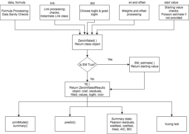
Algorithm flowchart
Classes and Methods
- LinkClass
- Instance Methods: link, link_inv, link_inv_deriv
- Classes Inheriting LinkClass: Logit, Probit, CLogLog, Cauchit, Log
- ZeroInflated
- Instance Methods:
- ziPoisson, ziNegBin, ziGeom
- gradPoisson, gradNegBin, gradGeom
- EM_estimate
- fit
- setter methods
- Static Methods:
- convert_params
- argument processing methods (dist, formula, link)
- Instance Methods:
- ZeroInflatedResults
- Instance methods: summary, printModel, predict, vcov
Usage
ZeroInflated(formula_str, df, params):
- Creates an instance of class ZeroInflated.
- Default params: dist = 'poisson', link = 'logit'
ZeroInflated(formula_str, df).fit(params):
- Returns an instance of class ZeroInflatedResults.
- Default params: EM = True, method = BFGS
ZeroInflated(formula_str, df).EM_estimate():
- Returns EM estimates of model as dict of pandas series.
ZeroInflated(formula_str, df).fit(params).method:
- method = summary, printModel, predict, vcov
Example dataset: DebTrivedi
Model for demand for medical care by elderly (ref.):
- 4406 indivduals aged 66 and above covered by medicare ('87/88 survey)
- Model demand for medicare: # of physician/non physician office and hospital visits ofp
- covariates for patients:
- hosp : # of hospital stays
- health: self perceived health status
- numchron: # of chronic conditions
- privins: private insurance indicator
- gender
- school
In [4]:
from zeroinfl import *


import numpy as np
import pandas as pd
from pandas.core import datetools

df = pd.read_csv('DebTrivedi.csv',index_col = [0])
sel = np.array([1, 6, 7, 8, 13, 15, 18])-1
df = df.iloc[:,sel]

formula_str = 'ofp ~ hosp + health + numchron + gender + school + privins | health'

import matplotlib.pyplot as plt
data_ofp = df.iloc[:,0].values.astype(int)
plt.hist(data_ofp, bins=np.arange(data_ofp.min(), data_ofp.max()), align = 'left', ec='black')
plt.xlabel('Number of physician office visits');plt.ylabel('Frequency')
plt.show()

Usage: printModel()
In [6]:
ZeroInflated(formula_str, df).fit().printModel()
Results from pscl package in R: print()
> model <- pscl::zeroinfl(ofp ~ health+gender+privins+hosp+numchron+school| health,
  data = dt, dist = 'poisson')
> print(model)
Call:
pscl::zeroinfl(formula = ofp ~ health + gender + privins + hosp + numchron + school | health,
    data = dt, dist = "poisson")

Count model coefficients (poisson with log link):
  (Intercept)   healthpoor  healthexcellent   gendermale   privinsyes     hosp
      1.39367      0.25420         -0.30775     -0.06486      0.08544  0.15913
     numchron       school
      0.10328      0.01959

Zero-inflation model coefficients (binomial with logit link):
    (Intercept)       healthpoor  healthexcellent
        -1.7336          -0.3992           0.4749
Usage: summary()
In [4]:
ZeroInflated(formula_str, df).fit().summary()
Results from pscl package in R: summary()
> summary(model)
Call:
pscl::zeroinfl(formula = ofp ~ health + gender + privins + hosp + numchron +
    school | health, data = dt, dist = "poisson")

Pearson residuals:
    Min      1Q  Median      3Q     Max
-2.5417 -1.2132 -0.4612  0.5889 25.1526

Count model coefficients (poisson with log link):
                 Estimate Std. Error z value Pr(>|z|)
(Intercept)      1.393672   0.024506  56.870  < 2e-16 ***
healthpoor       0.254201   0.017726  14.340  < 2e-16 ***
healthexcellent -0.307754   0.031428  -9.792  < 2e-16 ***
gendermale      -0.064859   0.013111  -4.947 7.54e-07 ***
privinsyes       0.085441   0.017310   4.936 7.97e-07 ***
hosp             0.159127   0.006059  26.262  < 2e-16 ***
numchron         0.103280   0.004736  21.806  < 2e-16 ***
school           0.019591   0.001885  10.395  < 2e-16 ***

Zero-inflation model coefficients (binomial with logit link):
                Estimate Std. Error z value Pr(>|z|)
(Intercept)     -1.73364    0.04809 -36.050  < 2e-16 ***
healthpoor      -0.39916    0.14655  -2.724  0.00646 **
healthexcellent  0.47490    0.14542   3.266  0.00109 **
---
Signif. codes:  0 '***' 0.001 '**' 0.01 '*' 0.05 '.' 0.1 ' ' 1

Number of iterations in BFGS optimization: 17
Log-likelihood: -1.629e+04 on 11 Df
Results
Zero Inflated Poisson: logit link
| Count: | Python | R |
|---|---|---|
| Intercept | 1.39367 | 1.39367 |
| health[T.excellent] | -0.30775 | -0.30775 |
| health[T.poor] | 0.25420 | 0.25420 |
| gender[T.male] | -0.06486 | -0.06486 |
| privins[T.yes] | 0.08544 | 0.08544 |
| hosp | 0.15913 | 0.15913 |
| numchron | 0.10328 | 0.10328 |
| school | 0.01959 | 0.01959 |
| Zero: | Python | R |
|---|---|---|
| Intercept | -1.73364 | -1.73364 |
| health[T.excellent] | 0.47490 | 0.47489 |
| health[T.poor] | -0.39916 | -0.39916 |
Results
Zero Inflated Geometric: logit link
| Count: | Python | R |
|---|---|---|
| Intercept | 0.92523 | 0.92523 |
| health[T.excellent] | -0.34160 | -0.34160 |
| health[T.poor] | 0.31351 | 0.31352 |
| gender[T.male] | -0.12678 | -0.12678 |
| privins[T.yes] | 0.22483 | 0.22483 |
| hosp | 0.22057 | 0.22057 |
| numchron | 0.17603 | 0.17603 |
| school | 0.02689 | 0.02689 |
| Zero: | Python | R |
|---|---|---|
| Intercept | -24.34361 | -24.33868 |
| health[T.excellent] | 10.00308 | 9.99858 |
| health[T.poor] | 19.44489 | 19.43996 |
Results
Zero Inflated Negative Binomial: logit link
| Count: | Python | R |
|---|---|---|
| Intercept | 0.94181 | 0.94206 |
| health[T.excellent] | -0.32944 | -0.32945 |
| health[T.poor] | 0.32891 | 0.32884 |
| gender[T.male] | -0.12468 | -0.12465 |
| privins[T.yes] | 0.21839 | 0.21832 |
| hosp | 0.22252 | 0.22250 |
| numchron | 0.17366 | 0.17363 |
| school | 0.02667 | 0.02667 |
| theta | 1.25876 | 1.25925 |
| Zero: | Python | R |
|---|---|---|
| Intercept | -5.04317 | -5.02321 |
| health[T.excellent] | 1.08234 | 1.06984 |
| health[T.poor] | 1.61952 | 1.60087 |
- Major:
- Summary statistics, predict()
- Vuong's Test
- Testing on 4 more datasets
- Minor:
- Dealing with missing values
- Functions docs
- Use standard names for ZeoInflatedResults class attributes (eg from python glm results class names)
- Exploring:
- Should ZeroInflatedResults class be inherited from ZeroInflated class
- Should ZeroInflated class be inherited from Loglikelihood class
- Future:
- Regularized optimization for ZIP, ZINB, ZIG
- Negative Binomial regression with joint estimation of theta and mu with variable weights.
- Use above for optimal EM estimation of starting values for ZINB.